ClusterProfiler富集分析
没想到一个富集分析涉及这么多的东西,今天没有完全的搞懂,先记录一下学习的代码 , 我打算先把R学一下,再来更新这篇文章
安装clusterProfiler等包
if (!requireNamespace("BiocManager", quietly = TRUE)) |
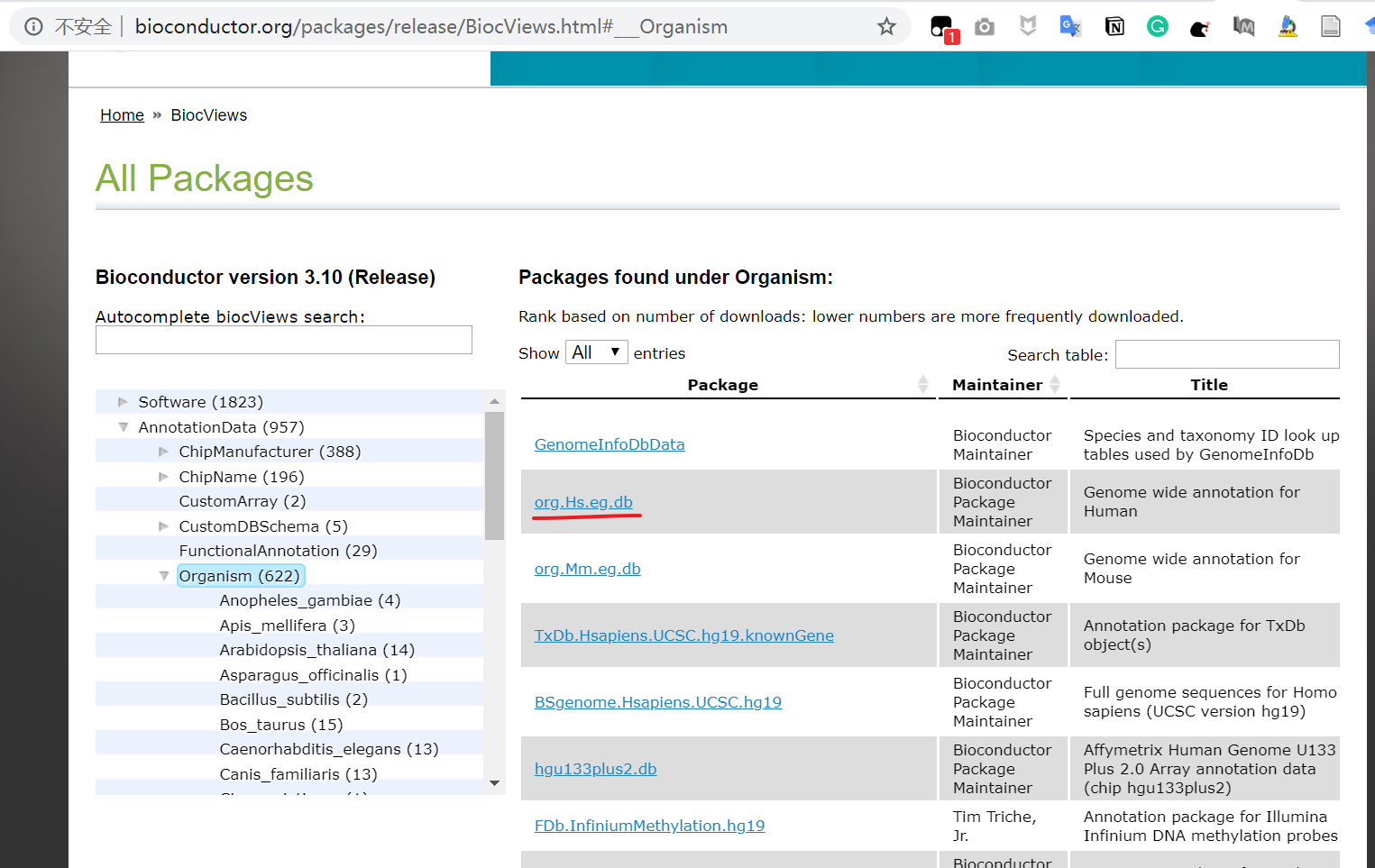
不同的参考物种,下载不同的数据:
加载R包
library(edgeR) |
数据导入
数据信息:
- 来源: TCGA Ovarian Serous Cystadenocarcinoma(OSC)
- 日期: 2017-06-14
- 下载工具: TCGABiolinks®
- 类型: RNA-seq(RSEM)
- 样本大小: 296
- 79 Immunoreactive(免疫反应物);
- 71 Mesenchymal(间充质);
- 67 Differentiated(分化);
- 79 Proliferative(增生);
表达量数据数据导入:
raw_count <- read.table("D:/baiduyundownload/富集分析/enrichment_analysis/TCGA_RNASeq_rawcounts.txt", |
查看部分数据
raw_count[1:5,1:5] |
分组信息导入
groups_df <- read.table("./RNASeq_classdefinitions.txt", |
差异表达分析
数据预过滤
根据CPM值,过滤低表达的基因. 标准是基因至少在50个样本量的表达量超过1
cpms <- cpm(raw_count) |
数据标准化和离散度(Dispersion)分析
创建DGEList类,用于存放表达量和样本信息
# create data structure to hold counts and subtype information for each sample. |
对原始文库数据计算标准化因子
#Normalize the data |
样本间距离
#create multidimensional scaling(MDS) plot. The command below will automatically |
计算离散度
#calculate dispersion |
差异表达分析
两样本使用exactTest即可.
多样本需要用
model.matrix,makeContrasts,glmFit,glmLRT等函数。
de <- exactTest(d, pair=c("Immunoreactive","Mesenchymal")) |
保存结果:
output_df <- cbind(gene=row.names(tt_exact_test), |
富集分析
读取数据
deg_df <- read.table("./edgeR_DEG.csv", |
数据预处理: 将基因列拆分
deg_df$symbol <- do.call(rbind, strsplit(deg_df$gene, "|", fixed = TRUE))[,1] |
GO分析
第一步: 筛选目标基因集。例如logFC >1, FDR < 0.05 认为是显著性上调
flt <- deg_df[deg_df$logFC > 1 & deg_df$FDR < 0.05,] |
第二步(1): GO富集分析
ego <- enrichGO(up_gene, |
第二步(2): KEGG富集分析
ekegg <- enrichKEGG(up_gene, |
第三步: 可视化
柱形图
barplot(ego, |
气泡图
dotplot(ego) |
dotplot(ekegg) |
View(as.data.frame(ekegg)) |
browseKEGG(ekegg, "hsa05224") |
GSEA分析
第一步: 构建排序基因表
rank_list <- deg_df$logFC |
第二步: GSEA分析
gseago <- gseGO(rank_list, |
第三步: 可视化
冒泡图
dotplot(gseakegg) |
GSEA图
View(as.data.frame(gseakegg)) |
enrichplot::gseaplot2(gseakegg, "hsa05224") |
Reference:
https://yulab-smu.github.io/clusterProfiler-book/index.html
https://guangchuangyu.github.io/software/clusterProfiler/documentation/
http://www.bioconductor.org/packages/release/BiocViews.html#___Organism
本博客所有文章除特别声明外,均采用 CC BY-NC-SA 4.0 许可协议。转载请注明来自 衷深学习!
 微信
微信 支付宝
支付宝
评论